Excel’s TAKE function allows you to extract the first, last, or specific columns or rows from a table. For example, you can extract data for the past three days or view the top ranked individuals. Let’s take a closer look at this.
The Excel TAKE function only works in Microsoft 365 or Excel for the web.
Prepare a table in Excel
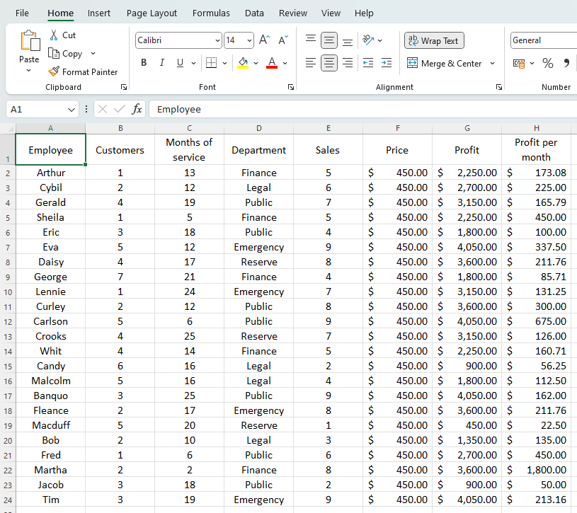
Before using TAKE and CHOOSE, the table must be formatted and named. Use this data table as an example.
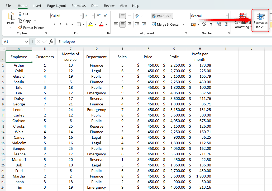
Make sure you include a row with column headings. Then select any cell in the table and click Format as Table in the Style group on the Home tab.
Click the layout you want, check “Table has header” in the dialog box that appears, and click OK.
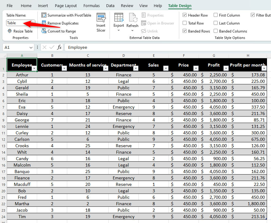
Now that Excel recognizes your data as a formatted table, you need to rename the table (for later use).of ribbon[テーブル デザイン]In the tab,[プロパティ]Go to group,[テーブル名]Change the fields as appropriate.
Now you are ready to extract data.
How to extract the first and/or last row and/or column in Excel using TAKE
The TAKE function in Excel is primarily used to extract the first or last few rows or columns from a table. The formula you need to use is:
=TAKE(X,Y,Z)
Where X is the table name, Y is the number of rows to extract, and Z is the number of columns to extract. Just put a ‘-‘ before Y or Z to change that part of the formula from the first row or column to the last row or column.
If the number of rows or columns to extract is likely to change, instead of entering numbers in Y and Z, you can enter the numbers in separate cells and enter the appropriate cell references.
In this example, we want to find the names of the top five employees based on monthly profits.
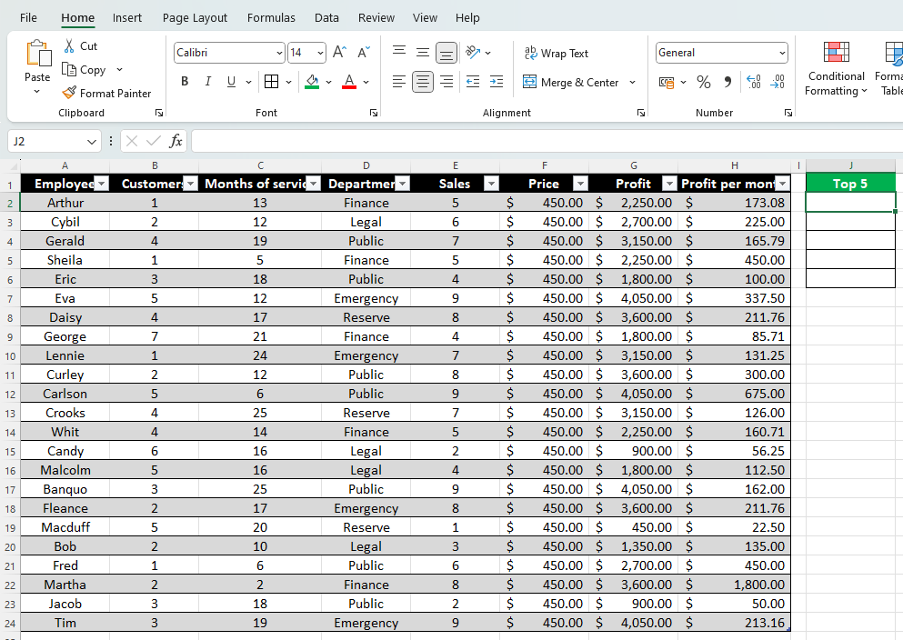
First, create a location on the worksheet to extract the data and enter the appropriate headers. In this example, we selected cell J2 and the header “Top 5”.
Then start typing the formula like this:
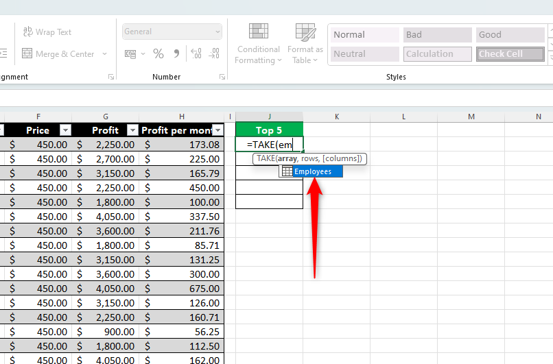
=TAKE(
The next part of the formula is the table name. Start typing the name of the table in the formula and double-click when the table name appears in the suggestion box. Then add a comma.
=TAKE(Employees,
Next, you need to tell Excel how many first or last rows to include in the extracted data. In our case, we want the top five employees. So, type “5” and add a comma. If you want the last 5 rows, enter -5. To extract all rows, add commas without numbers.
=TAKE(Employees,5,
Finally, finish the formula by telling Excel how many first or last columns to include. We only need the employee’s name, so select only the first column, close the parentheses, and press Enter. If you want to extract the last part, enter “-” again. X Column. To extract all columns, omit the number and press Enter.
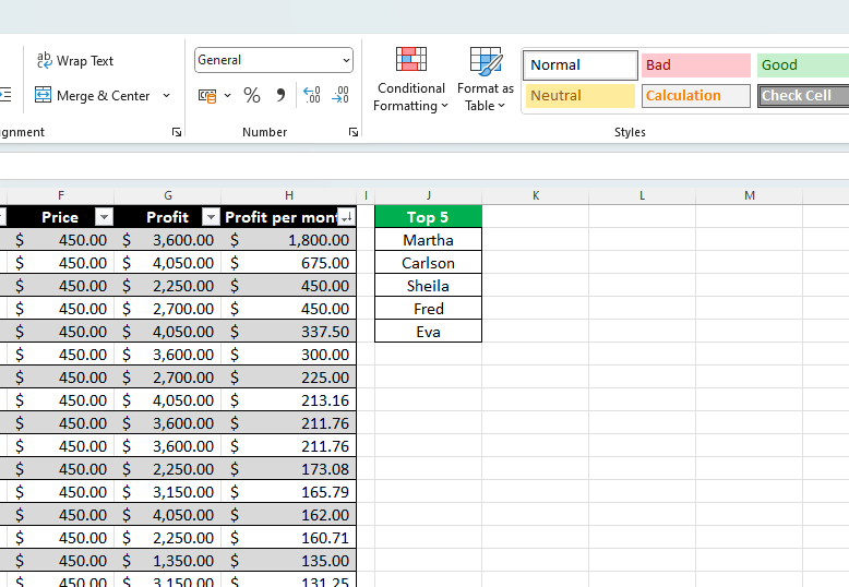
=TAKE(Employees,5,1)
Now you will see the desired result. Now, if you change or reorder the data in the table, his TAKE formula you just added will automatically adjust to extract the updated information. For example, let’s say you want to sort a column containing monthly profits.
If you add more data to the table, the TAKE expression will accommodate this. For example, if you add another employee’s data to an additional row at the bottom of the table (by dragging the table corner handle one row below his to complete the number), when searching for the criteria you set He includes this in his TAKE ceremony. .
How to extract specific columns in Excel using TAKE
If you want to extract a specific column, follow the steps above, but Add column names to the formula instead of column numbers.
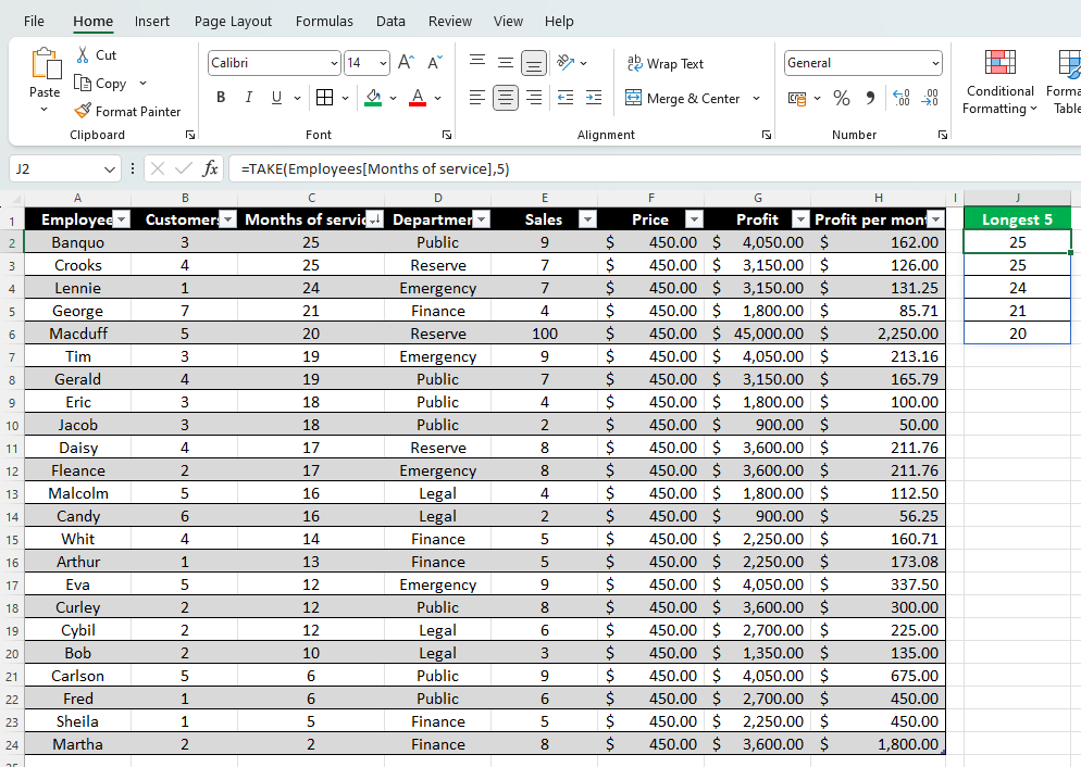
In the above example, suppose you want to calculate how many months of service each of the five longest-serving employees have had. This will be our formula:
=TAKE(Employees[Months of service],5)
Here “Employee” is the name of the table.[Months of service]” is the column name (note the lack of a comma between these two parts of the formula) and “5” is the number of rows to extract from the named column. Be sure to filter the corresponding column in the table. please.
How to use TAKE and AVERAGE in Excel
If you want to use TAKE with Excel’s AVERAGE function, follow the steps above, but Nest the TAKE expression inside the AVERAGE expression.
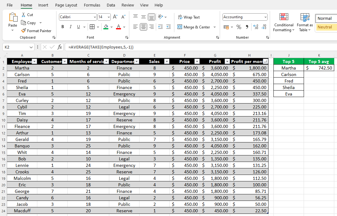
For example, suppose you want to calculate the average income of your top five employees. This will be our formula:
=AVERAGE(TAKE(Employees,5,-1))
Here, the AVERAGE expression surrounds the TAKE expression. The TAKE expression contains “Employees” (the table name), “5” (I want to get the top 5 rows), and “-1” (I want to get the last column).
Now you have a basic understanding of how the TAKE formula works in Excel. Go a step further and use Excel’s VSTACK and HSTACK functions to extract columns or rows from multiple ranges, or combine TAKE with Excel’s SORTBY function to work without reordering table columns. Now you can confirm that. Finally, you can use Excel’s DROP function. This function excludes specific cells and rows from the extracted data and works with exactly the same syntax as the TAKE function.


